The Blanchard (1985) Model of Perpetual Youth
This section analyzes a way to relax the standard assumption of infinite
lifetimes in the Ramsey/Cass-Koopmans
growth model. The trick, introduced by
Blanchard (1985)
Thus, an agent who has lived a thousand years is no more likely to die
in the next year than an agent who was born yesterday.
Time is measured continuously. If there is an instantaneous
probability d \pDies d t t t τ \tThen τ
ℵ t τ = e − d ( τ − t ) . \begin{gathered}\begin{aligned}
\Alive_{t}^{\tThen} & = e^{-\pDies(\tThen-t)} .
\end{aligned}\end{gathered} ℵ t τ = e − d ( τ − t ) . Assuming the instantaneous utility function is u ( c ) = log c \uFunc(c) = \log c u ( c ) = log c ϑ \timeRate ϑ t t t
∫ t ∞ ( log c τ ) e − ( ϑ + d ) ( τ − t ) d τ . \int_{t}^{\infty} (\log c_{\tThen}) e^{-(\timeRate+\pDies)(\tThen-t)} d\tThen. ∫ t ∞ ( log c τ ) e − ( ϑ + d ) ( τ − t ) d τ . where c τ c_{\tThen} c τ τ \tThen τ
ϑ ^ = ϑ + d . \begin{gathered}\begin{aligned}
\hat{\timeRate} & = \timeRate+\pDies.
\end{aligned}\end{gathered} ϑ ^ = ϑ + d . Answer:
A consumer with a pure time preference rate of zero will downweight
the utility he receives conditional on being alive by the probability
that he is still alive, yielding a discounted utility of
∫ t ∞ ( log c τ ) ℵ t τ e − ϑ ( τ − t ) d τ = ∫ t ∞ ( log c τ ) e − ϑ ( τ − t ) e − d ( τ − t ) d τ = ∫ t ∞ ( log c τ ) e − ( ϑ + d ) ( τ − t ) d τ = ∫ t ∞ ( log c τ ) e − ϑ ^ ( τ − t ) d τ \begin{gathered}\begin{aligned}
\int_{t}^{\infty} (\log c_{\tThen}) \Alive_{t}^{\tThen} e^{-\timeRate (\tThen-t)}d\tThen & = \int_{t}^{\infty} (\log c_{\tThen}) e^{-\timeRate (\tThen-t)} e^{-\pDies (\tThen-t)} d\tThen \\
& = \int_{t}^{\infty} (\log c_{\tThen}) e^{-(\timeRate+\pDies) (\tThen-t)} d\tThen
\\ & = \int_{t}^{\infty} (\log c_{\tThen}) e^{-\hat{\timeRate} (\tThen-t)} d\tThen
\end{aligned}\end{gathered} ∫ t ∞ ( log c τ ) ℵ t τ e − ϑ ( τ − t ) d τ = ∫ t ∞ ( log c τ ) e − ϑ ( τ − t ) e − d ( τ − t ) d τ = ∫ t ∞ ( log c τ ) e − ( ϑ + d ) ( τ − t ) d τ = ∫ t ∞ ( log c τ ) e − ϑ ^ ( τ − t ) d τ where ϑ ^ = ϑ + d \hat{\timeRate} = \timeRate+\pDies ϑ ^ = ϑ + d
A similar point holds in the discrete time model. A sensible thing to
assume is that if you have died before t + 1 t+1 t + 1
t + 1 t+1 t + 1
of death between T − 1 T-1 T − 1 T T T
V T − 1 = max u ( C T − 1 ) + ( 1 1 + ϑ ) u ( C T ) V_{T-1} = \max \uFunc(C_{T-1}) + \left(\frac{1}{1+\timeRate}\right) \uFunc(C_{T}) V T − 1 = max u ( C T − 1 ) + ( 1 + ϑ 1 ) u ( C T ) while if there is a probability d \pDies d T T T T + 1 T+1 T + 1
value would be:
V T − 1 = max u ( C T − 1 ) + ( 1 − d ) ( 1 1 + ϑ ) u ( C T ) + d β ⋅ 0 = max u ( C T − 1 ) + ( 1 − d 1 + ϑ ) u ( C T ) ≈ max u ( C T − 1 ) + ( 1 1 + ϑ + d ) u ( C T ) \begin{gathered}\begin{aligned}
V_{T-1} & = \max \uFunc(C_{T-1}) + (1-\pDies)\left(\frac{1}{1+\timeRate}\right) \uFunc(C_{T}) + \pDies \Discount \cdot 0
\\ & = \max \uFunc(C_{T-1}) + \left(\frac{1-\pDies}{1+\timeRate}\right) \uFunc(C_{T})
\\ & \approx \max \uFunc(C_{T-1}) + \left(\frac{1}{1+\timeRate+\pDies}\right) \uFunc(C_{T})
\end{aligned}\end{gathered} V T − 1 = max u ( C T − 1 ) + ( 1 − d ) ( 1 + ϑ 1 ) u ( C T ) + d β ⋅ 0 = max u ( C T − 1 ) + ( 1 + ϑ 1 − d ) u ( C T ) ≈ max u ( C T − 1 ) + ( 1 + ϑ + d 1 ) u ( C T ) But behavior in this case is virtually indistinguishable from the
behavior that would be induced if the consumer had a time preference
rate of ϑ + d \timeRate+\pDies ϑ + d
(6)
If the probability of death is constant, the expected remaining life
for an agent of any age is given by
∫ 0 ∞ d τ e − d τ d τ = d − 1 . \int_{0}^{\infty} \pDies \tau e^{-\pDies \tau}d\tau = \pDies^{-1}. ∫ 0 ∞ d τ e − d τ d τ = d − 1 . which we will call the agent’s ‘horizon.’ For example, if the chances
of dying per year are d = 1 / 50 \pDies=1/50 d = 1/50
We will assume that at every instant of time, a large cohort, whose size
is normalized to be d \pDies d
For an economy that has existed forever, explain why the
formula for the aggregate population at time t t t P t P_{t} P t
P t = d ∫ − ∞ t ℵ s t d s \begin{gathered}\begin{aligned}
P_{t} & = \pDies \int_{-\infty}^{t} \Alive_{s}^{\tNow} ds
\end{aligned}\end{gathered} P t = d ∫ − ∞ t ℵ s t d s and show that this formula implies that the population is P t = 1 P_{t}=1 P t = 1
Answer:
The aggregate population will be the sum of the still-alive persons
from all past generations.
The proportion of a population born at time s s s
at time τ \tThen τ ℵ s τ \Alive_{s}^{\tThen} ℵ s τ (1)
Thus, the absolute size at time τ \tThen τ d \pDies d
time s s s d ℵ s τ = d e − d ( τ − s ) \pDies \Alive_{s}^{\tThen} = \pDies e^{-\pDies (\tThen-s)} d ℵ s τ = d e − d ( τ − s )
total population will be the sum of the populations of all the cohorts
that are currently living. Since the economy has existed forever,
there will be remaining members of every cohort back to s = − ∞ s=-\infty s = − ∞
Thus, indexing each cohort by a time index s s s (8)
simply the sum of the populations of all currently living members of
every generation.
Substituting the formula for ℵ \Alive ℵ
P t = d ∫ − ∞ t e − d ( t − s ) d s = d ∫ t ∞ e − d ( s − t ) d s = d ∫ 0 ∞ e − d τ d τ = d d − 1 = 1 \begin{gathered}\begin{aligned}
P_{t} & = \pDies \int_{-\infty}^{t} e^{-\pDies(t-s)} ds
\\ & = \pDies \int_{t}^{\infty} e^{-\pDies(s-t)} ds
\\ & = \pDies \int_{0}^{\infty} e^{-\pDies \tThen}d\tThen
\\ & = \pDies \pDies^{-1}
\\ & = 1
\end{aligned}\end{gathered} P t = d ∫ − ∞ t e − d ( t − s ) d s = d ∫ t ∞ e − d ( s − t ) d s = d ∫ 0 ∞ e − d τ d τ = d d − 1 = 1 where the second line comes from a change of variables τ = s − t \tThen = s-t τ = s − t
and (9)
Now some notation. We will define variable x ( s , t ) x(s,t) x ( s , t ) t t t x x x s s s
Thus, c ( s , t ) c(s,t) c ( s , t ) t t t s s s
Suppose that the consumers in this economy do not have a bequest
motive. If they have positive assets at the instant when they die,
they are no happier than if they had zero assets. This means that if
someone were willing to pay them something while they are still alive
for the right to inherit their assets whenever they die, these consumers would
happily take that deal.
For a consumer with wealth w ( s , t ) w(s,t) w ( s , t ) d \pDies d d w ( s , t ) \pDies w(s,t) d w ( s , t ) w ( s , t ) w(s,t) w ( s , t ) d w ( s , t ) \pDies w(s,t) d w ( s , t )
But notice that from the standpoint of the consumer, this is
equivalent to saying that the interest rate received on wealth is
higher by amount d \pDies d
Now suppose the marginal product of capital in this
perfectly-competitive economy is constant at r \rfree r s s s t t t y ( s , t ) y(s,t) y ( s , t )
This plus the insurance scheme implies that the agent’s dynamic budget
constraint is given by
w ˙ ( s , t ) = ( r + d ) w ( s , t ) + y ( s , t ) − c ( s , t ) . \begin{gathered}\begin{aligned}
\dot{w}(s,t) & = (\rfree+\pDies) w(s,t) + y(s,t)-c(s,t) .
\end{aligned}\end{gathered} w ˙ ( s , t ) = ( r + d ) w ( s , t ) + y ( s , t ) − c ( s , t ) . Define the ‘effective’ interest rate as viewed by a consumer as r ^ = r + d \hat{\rfree} = \rfree+\pDies r ^ = r + d
Write the current-value Hamiltonian for the
individual’s maximization problem and use it to show that the growth
rate of consumption in period t t t s s s
( c ˙ ( s , t ) c ( s , t ) ) = r ^ − ϑ ^ = r − ϑ . \begin{gathered}\begin{aligned}
\left(\frac{\dot{c}(s,t)}{c(s,t)}\right) & = \hat{\rfree} - \hat{\timeRate}
\\ & = \rfree-\timeRate.
\end{aligned}\end{gathered} ( c ( s , t ) c ˙ ( s , t ) ) = r ^ − ϑ ^ = r − ϑ . Answer:
The current-value Hamiltonian is written
H ( c , w , λ ) = log c ( s , t ) + λ ( r ^ w ( s , t ) + y ( s , t ) − c ( s , t ) ) \Ham(c,w,\lambda) = \log c(s,t) + \lambda(\hat{\rfree} w(s,t) + y(s,t) - c(s,t)) H ( c , w , λ ) = log c ( s , t ) + λ ( r ^ w ( s , t ) + y ( s , t ) − c ( s , t )) so the first optimality condition ∂ H / ∂ c ( s , t ) = 0 \partial \Ham/\partial c(s,t) = 0 ∂ H / ∂ c ( s , t ) = 0
1 / c ( s , t ) = λ − c ˙ ( s , t ) / c ( s , t ) 2 = λ ˙ \begin{gathered}\begin{aligned}
1/c(s,t) & = \lambda
\\ - \dot{c}(s,t)/c(s,t)^{2} & = \dot{\lambda}
\end{aligned}\end{gathered} 1/ c ( s , t ) − c ˙ ( s , t ) / c ( s , t ) 2 = λ = λ ˙ and the second optimization condtion implies
λ ˙ = ϑ ^ λ − ∂ H / ∂ w ( s , t ) = ϑ ^ λ − r ^ λ ( λ ˙ λ ) = ϑ ^ − r ^ ( − c ˙ ( s , t ) c ( s , t ) c ( s , t ) 2 ) = ϑ ^ − r ^ ( c ˙ ( s , t ) c ( s , t ) ) = r ^ − ϑ ^ = r − ϑ . \begin{gathered}\begin{aligned}
\dot{\lambda} & = \hat{\timeRate} \lambda - \partial \Ham/\partial w(s,t)
\\ & = \hat{\timeRate} \lambda - \hat{\rfree} \lambda
\\ \left(\frac{\dot{\lambda}}{\lambda}\right) & = \hat{\timeRate}-\hat{\rfree}
\\ \left(\frac{-\dot{c}(s,t) c(s,t)}{c(s,t)^{2}}\right) & = \hat{\timeRate}-\hat{\rfree}
\\ \left(\frac{\dot{c}(s,t)}{c(s,t)}\right) & = \hat{\rfree}-\hat{\timeRate}
\\ & = \rfree-\timeRate .
\end{aligned}\end{gathered} λ ˙ ( λ λ ˙ ) ( c ( s , t ) 2 − c ˙ ( s , t ) c ( s , t ) ) ( c ( s , t ) c ˙ ( s , t ) ) = ϑ ^ λ − ∂ H / ∂ w ( s , t ) = ϑ ^ λ − r ^ λ = ϑ ^ − r ^ = ϑ ^ − r ^ = r ^ − ϑ ^ = r − ϑ . Use the first order condition for consumption and the
intertemporal budget constraint implied by (10) t t t s s s
c ( s , t ) = ϑ ^ ( w ( s , t ) + h ( s , t ) ) c(s,t) = \hat{\timeRate}(w(s,t)+h(s,t)) c ( s , t ) = ϑ ^ ( w ( s , t ) + h ( s , t )) where recall that ϑ ^ = ϑ + d \hat{\timeRate}=\timeRate+\pDies ϑ ^ = ϑ + d
h ( s , t ) = ∫ t ∞ ( y ( s , τ ) / R ^ t τ ) d τ h(s,t) = \int_{t}^{\infty} \left(y(s,\tThen)/\hat{\mathcal{R}}_{t}^{\tThen}\right) d\tThen h ( s , t ) = ∫ t ∞ ( y ( s , τ ) / R ^ t τ ) d τ where
R ^ t τ = e ∫ t τ ( r μ + d ) d μ \begin{gathered}\begin{aligned}
\hat{\mathcal{R}}_{t}^{\tThen} & = e^{\int_{t}^{\tThen} (\rfree_{\mu}+\pDies) d\mu}
\end{aligned}\end{gathered} R ^ t τ = e ∫ t τ ( r μ + d ) d μ (this is simply the compound discount factor necessary to take
account of time-varying interest rates; if interest rates are
constant at r \rfree r e − r ( τ − t ) e^{-\rfree(\tThen-t)} e − r ( τ − t )
Answer:
The IBC says that the PDV of consumption must equal wealth plus the PDV
of future labor income:
∫ t ∞ ( c ( s , τ ) / R ^ t τ ) d τ = w ( s , t ) + ∫ t ∞ y ( τ , t ) / R ^ t τ d τ ∫ t ∞ ( c ( s , τ ) / R ^ t τ ) d τ = w ( s , t ) + h ( s , t ) . \begin{gathered}\begin{aligned}
\int_{t}^{\infty} (c(s,\tThen)/\hat{\mathcal{R}}_{t}^{\tThen}) d\tThen & = w(s,t) + \int_{t}^{\infty} y(\tThen,t)/\hat{\mathcal{R}}_{t}^{\tThen} d\tThen
\\ \int_{t}^{\infty} (c(s,\tThen)/\hat{\mathcal{R}}_{t}^{\tThen}) d\tThen & = w(s,t) + h(s,t).
\end{aligned}\end{gathered} ∫ t ∞ ( c ( s , τ ) / R ^ t τ ) d τ ∫ t ∞ ( c ( s , τ ) / R ^ t τ ) d τ = w ( s , t ) + ∫ t ∞ y ( τ , t ) / R ^ t τ d τ = w ( s , t ) + h ( s , t ) . But if c ˙ ( s , t ) / c ( s , t ) = r ^ t − ϑ ^ \dot{c}(s,t)/c(s,t) = \hat{\rfree}_{t}-\hat{\timeRate} c ˙ ( s , t ) / c ( s , t ) = r ^ t − ϑ ^
c ( s , τ ) = c ( s , t ) e ∫ s τ r ^ μ d μ e − ϑ ^ ( τ − t ) \begin{gathered}\begin{aligned}
c(s,\tThen) & = c(s,t)e^{\int_{s}^{\tThen}\hat{\rfree}_\mu d\mu}e^{-\hat{\timeRate}(\tThen-t)}
\end{aligned}\end{gathered} c ( s , τ ) = c ( s , t ) e ∫ s τ r ^ μ d μ e − ϑ ^ ( τ − t ) implying
∫ t ∞ ( c ( s , τ ) / R ^ t τ ) d τ = ∫ t ∞ c ( s , t ) e ∫ s τ r ^ μ d μ e − ϑ ^ ( τ − t ) e − ∫ s τ r ^ μ d μ d τ = c ( s , t ) ∫ t ∞ e − ϑ ^ ( τ − t ) d τ = c ( s , t ) / ϑ ^ \begin{gathered}\begin{aligned}
\int_{t}^{\infty} (c(s,\tThen)/\hat{\mathcal{R}}_{t}^{\tThen}) d\tThen & =
\int_{t}^{\infty} c(s,t) e^{\int_{s}^{\tThen}\hat{\rfree}_\mu d\mu}e^{-\hat{\timeRate}(\tThen-t)}e^{-\int_{s}^{\tThen}\hat{\rfree}_\mu d\mu} d\tThen
\\ & = c(s,t) \int_{t}^{\infty} e^{-\hat{\timeRate}(\tThen-t)} d\tThen
\\ & = c(s,t)/\hat{\timeRate}
\end{aligned}\end{gathered} ∫ t ∞ ( c ( s , τ ) / R ^ t τ ) d τ = ∫ t ∞ c ( s , t ) e ∫ s τ r ^ μ d μ e − ϑ ^ ( τ − t ) e − ∫ s τ r ^ μ d μ d τ = c ( s , t ) ∫ t ∞ e − ϑ ^ ( τ − t ) d τ = c ( s , t ) / ϑ ^ so that the IBC becomes:
c ( s , t ) / ϑ ^ = w ( s , t ) + h ( s , t ) c ( s , t ) = ϑ ^ ( w ( s , t ) + h ( s , t ) ) . \begin{gathered}\begin{aligned}
c(s,t)/\hat{\timeRate} & = w(s,t)+h(s,t) \\
c(s,t) & = \hat{\timeRate} (w(s,t)+h(s,t)) .
\end{aligned}\end{gathered} c ( s , t ) / ϑ ^ c ( s , t ) = w ( s , t ) + h ( s , t ) = ϑ ^ ( w ( s , t ) + h ( s , t )) . Suppose we define upper-case variables as the aggregate value across all
generations currently living of the corresponding lower-case value, e.g.
aggregate consumption is
C ( t ) = ∫ − ∞ t d c ( τ , t ) ℵ τ t d τ . \begin{gathered}\begin{aligned}
C(t) & = \int_{-\infty}^{t} \pDies c(\tThen,t) \Alive_{\tThen}^{t} d\tThen.
\end{aligned}\end{gathered} C ( t ) = ∫ − ∞ t d c ( τ , t ) ℵ τ t d τ . (Easy) Show that the aggregate level of consumption in
this economy is
C ( t ) = ϑ ^ ( W ( t ) + H ( t ) ) . \begin{gathered}\begin{aligned}
C(t) & = \hat{\timeRate} (W(t) + H(t)) .
\end{aligned}\end{gathered} C ( t ) = ϑ ^ ( W ( t ) + H ( t )) . Answer:
C ( t ) = ∫ − ∞ t d c ( τ , t ) ℵ τ t d τ = ∫ − ∞ t d ϑ ^ ( w ( τ , t ) + h ( τ , t ) ) ℵ τ t d τ = ϑ ^ ( W ( t ) + H ( t ) ) \begin{gathered}\begin{aligned}
C(t) & = \int_{-\infty}^{t} \pDies c(\tThen,t) \Alive_{\tThen}^{t} d\tThen \\
& = \int_{-\infty}^{t} \pDies \hat{\timeRate}(w(\tThen,t)+h(\tThen,t)) \Alive_{\tThen}^{t} d\tThen \\
& = \hat{\timeRate} (W(t)+H(t))
\end{aligned}\end{gathered} C ( t ) = ∫ − ∞ t d c ( τ , t ) ℵ τ t d τ = ∫ − ∞ t d ϑ ^ ( w ( τ , t ) + h ( τ , t )) ℵ τ t d τ = ϑ ^ ( W ( t ) + H ( t )) from the definition of W ( t ) W(t) W ( t ) H ( t ) H(t) H ( t )
Suppose all living agents in this economy receive the same noncapital
income, y ( s , t ) = Y ( t ) y(s,t) = Y(t) y ( s , t ) = Y ( t ) Y ( t ) Y(t) Y ( t ) t t t
H ( t ) = ∫ t ∞ ( Y ( τ ) / R ^ t τ ) d τ \begin{gathered}\begin{aligned}
H(t) & = \int_{t}^{\infty} (Y(\tThen)/\hat{\mathcal{R}}_{t}^{\tThen}) d\tThen
\end{aligned}\end{gathered} H ( t ) = ∫ t ∞ ( Y ( τ ) / R ^ t τ ) d τ where
H ˙ ( t ) = r ^ t H ( t ) − Y ( t ) . \begin{gathered}\begin{aligned}
\dot{H}(t) & = \hat{\rfree}_{t} H(t) - Y(t) .
\end{aligned}\end{gathered} H ˙ ( t ) = r ^ t H ( t ) − Y ( t ) . The differential equation for aggregate wealth can be
shown to be
W ˙ ( t ) = w ( t , t ) − d W ( t ) + ∫ − ∞ t w ˙ ( τ , t ) d e − d ( t − τ ) d τ , \begin{gathered}\begin{aligned}
\dot{W}(t) & = w(t,t) - \pDies W(t) + \int_{-\infty}^{t} \dot{w}(\tThen,t) \pDies e^{-\pDies(t-\tThen)} d\tThen,
\end{aligned}\end{gathered} W ˙ ( t ) = w ( t , t ) − d W ( t ) + ∫ − ∞ t w ˙ ( τ , t ) d e − d ( t − τ ) d τ , where w ( t , t ) = 0 w(t,t)=0 w ( t , t ) = 0 d W ( t ) \pDies W(t) d W ( t ) (10)
∫ − ∞ t w ˙ ( τ , t ) d e − d ( t − τ ) d τ = ( r + d ) W ( t ) + Y ( t ) − C ( t ) \begin{gathered}\begin{aligned}
\int_{-\infty}^{t} \dot{w}(\tThen,t) \pDies e^{-\pDies(t-\tThen)} d\tThen & = (\rfree+\pDies) W(t) + Y(t)-C(t)
\end{aligned}\end{gathered} ∫ − ∞ t w ˙ ( τ , t ) d e − d ( t − τ ) d τ = ( r + d ) W ( t ) + Y ( t ) − C ( t ) so (27)
W ˙ ( t ) = r W ( t ) + Y ( t ) − C ( t ) . \begin{gathered}\begin{aligned}
\dot{W}(t) & = \rfree W(t) + Y(t)-C(t).
\end{aligned}\end{gathered} W ˙ ( t ) = r W ( t ) + Y ( t ) − C ( t ) . Collecting, writing out r ^ = r + d \hat{\rfree}=\rfree+\pDies r ^ = r + d ϑ ^ = ϑ + d \hat{\timeRate}=\timeRate+\pDies ϑ ^ = ϑ + d ( t ) (t) ( t )
C = ( d + ϑ ) ( H + W ) H ˙ = ( r + d ) H − Y W ˙ = r W + Y − C \begin{gathered}\begin{aligned}
C & = (\pDies+\timeRate) (H+W) \\
\dot{H} & = (\rfree+\pDies) H - Y \\
\dot{W} & = \rfree W + Y - C
\end{aligned}\end{gathered} C H ˙ W ˙ = ( d + ϑ ) ( H + W ) = ( r + d ) H − Y = r W + Y − C Use these equations to show that in this economy
C ˙ = ( r − ϑ ) C − d ( d + ϑ ) W \begin{gathered}\begin{aligned}
\dot{C} & = (\rfree-\timeRate) C - \pDies(\pDies+\timeRate) W
\end{aligned}\end{gathered} C ˙ = ( r − ϑ ) C − d ( d + ϑ ) W Hint: Differentiate (30) H H H (30) H H H
Answer:
Time differentiate (30) H ˙ \dot{H} H ˙
W ˙ \dot{W} W ˙ H H H
C ˙ = ( d + ϑ ) [ ( r + d ) H − Y + r W + Y − C ] = ( d + ϑ ) [ ( r + d ) H + r W ] − C ( d + ϑ ) = ( d + ϑ ) [ ( r + d ) ( C d + ϑ − W ) + r W ] − C ( d + ϑ ) = ( r + d ) C + ( d + ϑ ) [ r W − ( r + d ) W ] − C ( d + ϑ ) = ( r − ϑ ) C − ( d + ϑ ) d W . \begin{gathered}\begin{aligned}
\dot{C} & = (\pDies+\timeRate)\left[(\rfree+\pDies) H - Y + \rfree W + Y - C\right]
\\ & = (\pDies+\timeRate)\left[(\rfree+\pDies) H + \rfree W \right] - C (\pDies+\timeRate)
\\ & = (\pDies+\timeRate)\left[(\rfree+\pDies) \left(\frac{C}{\pDies+\timeRate}-W\right)+r W\right] - C (\pDies+\timeRate)
\\ & = (\rfree+\pDies) C + (\pDies+\timeRate)\left[ rW - (\rfree+\pDies) W \right] - C(\pDies+\timeRate)
\\ & = (\rfree-\timeRate) C - (\pDies+\timeRate)\pDies W.
\end{aligned}\end{gathered} C ˙ = ( d + ϑ ) [ ( r + d ) H − Y + r W + Y − C ] = ( d + ϑ ) [ ( r + d ) H + r W ] − C ( d + ϑ ) = ( d + ϑ ) [ ( r + d ) ( d + ϑ C − W ) + r W ] − C ( d + ϑ ) = ( r + d ) C + ( d + ϑ ) [ r W − ( r + d ) W ] − C ( d + ϑ ) = ( r − ϑ ) C − ( d + ϑ ) d W . Now assume there is a standard production function
F ( K ) = K α − δ K \FFunc(K)=K^{\alpha}-\delta K F ( K ) = K α − δK r r r
r = F ′ ( K ) = α K α − 1 − δ \rfree = \FFunc^{\prime}(K) = \alpha K^{\alpha-1}-\delta r = F ′ ( K ) = α K α − 1 − δ and the aggregate capital stock at time t t t K ( t ) = W ( t ) K(t)=W(t) K ( t ) = W ( t )
K ˙ = K α − δ K − C . \begin{gathered}\begin{aligned}
\dot{K} & = K^{\alpha}-\delta K -C.
\end{aligned}\end{gathered} K ˙ = K α − δK − C . Show that the following equation
d ( d + ϑ ) K = C ( α K α − 1 − δ − ϑ ) \begin{gathered}\begin{aligned}
\pDies(\pDies+\timeRate) K & = C(\alpha K^{\alpha-1}-\delta-\timeRate)
\end{aligned}\end{gathered} d ( d + ϑ ) K = C ( α K α − 1 − δ − ϑ ) describes the C ˙ = 0 \dot{C}=0 C ˙ = 0
lim C → 0 K = 0 lim C → ∞ K = ( ( ϑ + δ ) / α ) 1 / α − 1 . \begin{gathered}\begin{aligned}
\lim_{C \rightarrow 0} K & = 0
\\ \lim_{C \rightarrow \infty} K & = ((\timeRate+\delta)/\alpha)^{1/{\alpha-1}}.
\end{aligned}\end{gathered} C → 0 lim K C → ∞ lim K = 0 = (( ϑ + δ ) / α ) 1/ α − 1 . Answer:
Rewriting the C ˙ \dot{C} C ˙ K K K
C ˙ = ( α K α − 1 − ϑ − δ ) C − ( d + ϑ ) d K . \begin{gathered}\begin{aligned}
\dot{C} & = (\alpha K^{\alpha-1} - \timeRate - \delta)C - (\pDies+\timeRate)\pDies K.
\end{aligned}\end{gathered} C ˙ = ( α K α − 1 − ϑ − δ ) C − ( d + ϑ ) d K . The C ˙ = 0 \dot{C}=0 C ˙ = 0
0 = ( α K α − 1 − ϑ − δ ) − d ( d + ϑ ) K / C d ( d + ϑ ) K / C = ( α K α − 1 − δ − ϑ ) d ( d + ϑ ) K = C ( α K α − 1 − δ − ϑ ) \begin{gathered}\begin{aligned}
0 & = (\alpha K^{\alpha-1}-\timeRate-\delta) - \pDies(\pDies+\timeRate) K/C
\\ \pDies(\pDies+\timeRate) K/C & = (\alpha K^{\alpha-1}-\delta-\timeRate)
\\ \pDies(\pDies+\timeRate) K & = C(\alpha K^{\alpha-1}-\delta-\timeRate)
\end{aligned}\end{gathered} 0 d ( d + ϑ ) K / C d ( d + ϑ ) K = ( α K α − 1 − ϑ − δ ) − d ( d + ϑ ) K / C = ( α K α − 1 − δ − ϑ ) = C ( α K α − 1 − δ − ϑ ) In the limit as C → 0 C \rightarrow 0 C → 0
d ( d + ϑ ) K = 0 \pDies(\pDies+\timeRate) K = 0 d ( d + ϑ ) K = 0 which can be true only if lim { C → 0 } K = 0 \lim_{\{C \rightarrow 0\}} K = 0 lim { C → 0 } K = 0
On the other hand, as C → ∞ C \rightarrow \infty C → ∞ K K K
must remain finite (because the DBC does not allow infinite
accumulation of K K K K K K
could never be paid for by a production function with diminishing marginal returns), which means that
lim { C → ∞ } α K α − 1 = ( ϑ + δ ) K ∗ = ( ( ϑ + δ ) / α ) 1 / α − 1 . \begin{gathered}\begin{aligned}
\lim_{\{C \rightarrow \infty\}} \alpha K^{\alpha-1} & = (\timeRate+\delta)
\\ K^{*} & = ((\timeRate+\delta)/\alpha)^{1/{\alpha-1}}.
\end{aligned}\end{gathered} { C → ∞ } lim α K α − 1 K ∗ = ( ϑ + δ ) = (( ϑ + δ ) / α ) 1/ α − 1 . Using your results from the previous question and the aggregate
dynamic budget constraint, draw the phase diagram for this model and
discuss how and why it differs from the phase diagram for the
standard Ramsey-Cass/Koopmans model. (please use K ∗ K^{*} K ∗ RCK steady-state capital stock and K ˉ \bar{K} K ˉ K K K
Answer:
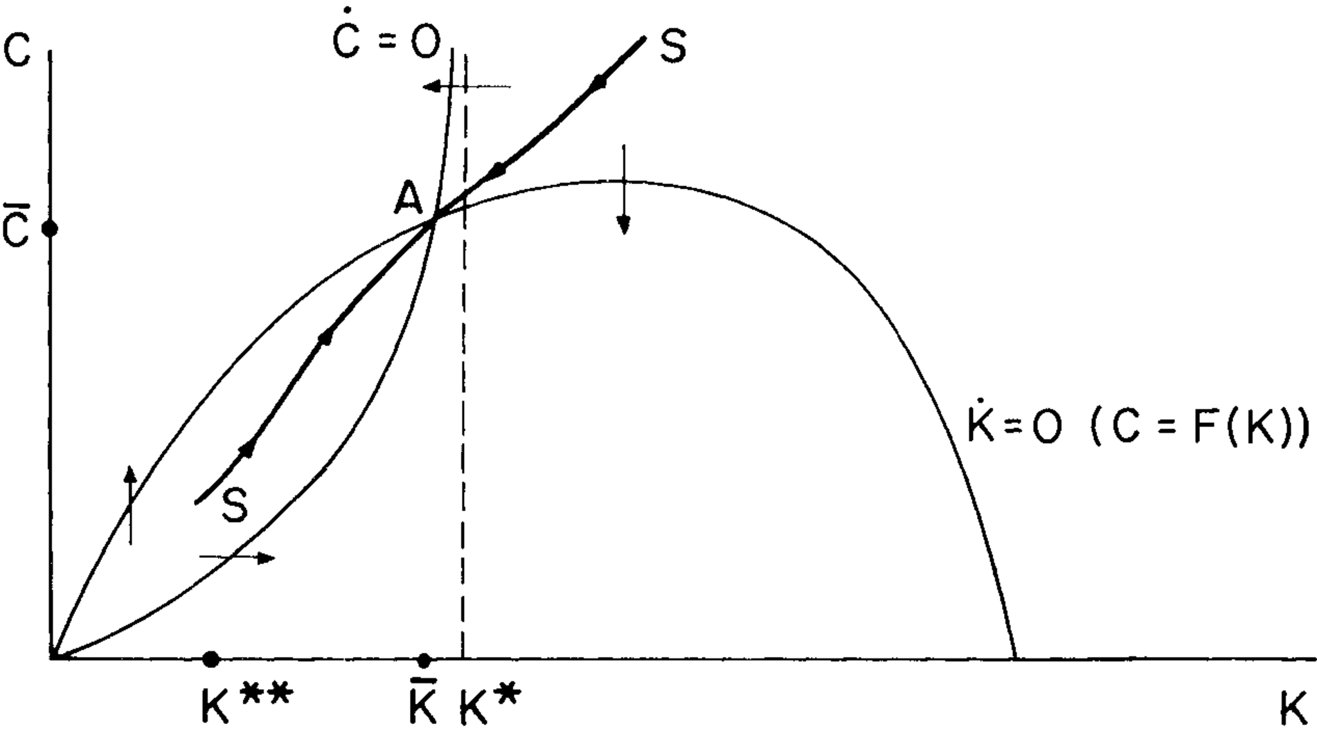
Using (34) K ˙ = 0 \dot{K}=0 K ˙ = 0
C = K α − δ K \begin{gathered}\begin{aligned}
C & = K^{\alpha}-\delta K
\end{aligned}\end{gathered} C = K α − δK which yields the usual hump-shaped K ˙ = 0 \dot{K}=0 K ˙ = 0
Rewriting the C ˙ \dot{C} C ˙ K K K
C ˙ = ( α K α − 1 − ϑ − δ ) C − ( d + ϑ ) d K . \begin{gathered}\begin{aligned}
\dot{C} & = (\alpha K^{\alpha-1} - \timeRate - \delta)C - (\pDies+\timeRate)\pDies K.
\end{aligned}\end{gathered} C ˙ = ( α K α − 1 − ϑ − δ ) C − ( d + ϑ ) d K . The C ˙ = 0 \dot{C}=0 C ˙ = 0
0 = ( α K α − 1 − ϑ − δ ) − d ( d + ϑ ) K / C d ( d + ϑ ) K / C = ( α K α − 1 − δ − ϑ ) d ( d + ϑ ) K = C ( α K α − 1 − δ − ϑ ) \begin{gathered}\begin{aligned}
0 & = (\alpha K^{\alpha-1}-\timeRate-\delta) - \pDies(\pDies+\timeRate) K/C
\\ \pDies(\pDies+\timeRate) K/C & = (\alpha K^{\alpha-1}-\delta-\timeRate)
\\ \pDies(\pDies+\timeRate) K & = C(\alpha K^{\alpha-1}-\delta-\timeRate)
\end{aligned}\end{gathered} 0 d ( d + ϑ ) K / C d ( d + ϑ ) K = ( α K α − 1 − ϑ − δ ) − d ( d + ϑ ) K / C = ( α K α − 1 − δ − ϑ ) = C ( α K α − 1 − δ − ϑ ) In the limit as C → 0 C \rightarrow 0 C → 0
d ( d + ϑ ) K = 0 \pDies(\pDies+\timeRate) K = 0 d ( d + ϑ ) K = 0 which can be true only if lim { C → 0 } K = 0 \lim_{\{C \rightarrow 0\}} K = 0 lim { C → 0 } K = 0
On the other hand, as C → ∞ C \rightarrow \infty C → ∞ K K K
must remain finite (because the DBC does not allow infinite
accumulation of K K K
lim { C → ∞ } α K α − 1 = ( ϑ + δ ) K ∗ = ( ( ϑ + δ ) / α ) 1 / ( α − 1 ) . \begin{gathered}\begin{aligned}
\lim_{\{C \rightarrow \infty\}} \alpha K^{\alpha-1} & = (\timeRate+\delta)
\\ K^{*} & = ((\timeRate+\delta)/\alpha)^{1/{(\alpha-1)}}.
\end{aligned}\end{gathered} { C → ∞ } lim α K α − 1 K ∗ = ( ϑ + δ ) = (( ϑ + δ ) / α ) 1/ ( α − 1 ) . In the infinite horizon economy we have d = 0 \pDies = 0 d = 0
steady-state interest rate would be the K ∗ K^{*} K ∗ α K α − 1 − δ = ϑ \alpha K^{\alpha-1}-\delta = \timeRate α K α − 1 − δ = ϑ K / C K/C K / C d ( d + ϑ ) \pDies(\pDies+\timeRate) d ( d + ϑ )
strictly positive, in this finite-horizon economy we would have
C ˙ / C < 0 \dot{C}/C < 0 C ˙ / C < 0 K = K ∗ K=K^{*} K = K ∗
for (38) α K α − 1 \alpha K^{\alpha-1} α K α − 1
to be larger than it is at K ∗ K^{*} K ∗
steady-state interest rate, and thus we need a lower steady-state
capital stock, which is depicted in the figure as K ˉ \bar{K} K ˉ
This makes sense because the finite-horizon consumers in this economy
discount the future more than the representative agent does, because
they die but a representative agent does not.
These results are combined in the figure, which shows that the intersection
of the C ˙ = 0 \dot{C}=0 C ˙ = 0 K ˙ = 0 \dot{K}=0 K ˙ = 0 A A A
which corresponds to a lower level of the capital stock than in the
infinite horizon model.
Now consider the introduction of a government that finances spending
either by lump-sum taxes or by debt. Its dynamic budget constraint is
D ˙ = r D + G − T \dot{D} = \rfree D + G - \TaxLev D ˙ = r D + G − T where D D D G G G T \TaxLev T
R t s = e ∫ t s r v d v \begin{gathered}\begin{aligned}
\mathcal{R}_t^{s} = e^{\int_t^{s}\rfree_v dv}
\end{aligned}\end{gathered} R t s = e ∫ t s r v d v as the compound interest factor between time t t t s s s
lim t → ∞ D t / R t s = 0. \lim_{t \rightarrow \infty} D_t/\mathcal{R}_t^{s} = 0. t → ∞ lim D t / R t s = 0. Consider the following fiscal policy experiment. Until time t t t G s = D s = T s = 0 ∀ s < t G_s = D_s = \TaxLev_s=0~\forall~s<t G s = D s = T s = 0 ∀ s < t t t t D D D D ˙ = 0 \dot{D}=0 D ˙ = 0 D D D
W = K + D Y = Y − T H = ∫ t ∞ Y / R ^ t s d s \begin{gathered}\begin{aligned}
\mathcal{W} & = K + D
\\ \mathcal{Y} & = Y - \TaxLev
\\ \mathcal{H} & = \int_{t}^{\infty} \mathcal{Y}/\hat{\mathcal{R}}_{t}^{s} ds
\end{aligned}\end{gathered} W Y H = K + D = Y − T = ∫ t ∞ Y / R ^ t s d s Explain why the effect of this policy is to modify the aggregate
specification of the economy to
C = ( d + ϑ ) ( H + W ) W ˙ = r W + Y − C H ˙ = ( r + d ) H − Y \begin{gathered}\begin{aligned}
C & = (\pDies+\timeRate) (\mathcal{H} + \mathcal{W})
\\ \dot{\mathcal{W}} & = \rfree \mathcal{W} + \mathcal{Y}- C
\\ \dot{\mathcal{H}} & = (\rfree+\pDies) \mathcal{H} - \mathcal{Y}
\end{aligned}\end{gathered} C W ˙ H ˙ = ( d + ϑ ) ( H + W ) = r W + Y − C = ( r + d ) H − Y Answer:
The effect of the government policy is twofold. On the one hand,
the distribution of government bonds increases the consumers’
wealth W W W
resulting in a new definition of wealth W \mathcal{W} W
includes the bonds. On the other hand, the higher value of taxes
off to infinity reduces the consumers’ human wealth by an amount
equal to the present discounted value of the taxes.
The change in (redefined) wealth is now net income Y − ϑ Y-\timeRate Y − ϑ
minus consumption.
Use these equations to show that the new dynamic equations for
the economy are
C ˙ = ( r − ϑ ) C − d ( d + ϑ ) ( K + D ) K ˙ = K α − δ K − C \begin{gathered}\begin{aligned}
\dot{C} & = (\rfree - \timeRate)C - \pDies(\pDies+\timeRate)(K+D)
\\ \dot{K} & = K^{\alpha}-\delta K - C
\end{aligned}\end{gathered} C ˙ K ˙ = ( r − ϑ ) C − d ( d + ϑ ) ( K + D ) = K α − δK − C Show how the policy change affects the economy over time, using a
phase diagram and a diagram showing the dynamics of aggregate
consumption after the policy is introduced. Explain the impact
of the policy on different generations in the economy.
Answer:
Time differentiating (50)
C ˙ = ( d + ϑ ) ( H ˙ + W ˙ ) = ( d + ϑ ) ( r W + ( r + d ) H − C ) \begin{gathered}\begin{aligned}
\dot{C} & = (\pDies+\timeRate) (\dot{\mathcal{H}} + \dot{\mathcal{W}})
\\ & = (\pDies+\timeRate)(\rfree \mathcal{W}+(\rfree+\pDies)\mathcal{H}-C)
\end{aligned}\end{gathered} C ˙ = ( d + ϑ ) ( H ˙ + W ˙ ) = ( d + ϑ ) ( r W + ( r + d ) H − C ) Now solve (50) H \mathcal{H} H
H = ( C d + ϑ ) − W \begin{gathered}\begin{aligned}
\mathcal{H} & = \left(\frac{C}{\pDies+ \timeRate}\right)-\mathcal{W}
\end{aligned}\end{gathered} H = ( d + ϑ C ) − W and substitute into (52)
C ˙ = ( d + ϑ ) ( r W + ( r + d ) ( C ( d + ϑ ) − 1 − W ) − C ) = ( r + d ) C − ( d + ϑ ) C − d ( d + ϑ ) W = ( r − ϑ ) C − d ( d + ϑ ) ( K + D ) . \begin{gathered}\begin{aligned}
\dot{C} & = (\pDies+\timeRate)(\rfree \mathcal{W}+(\rfree+\pDies)(C(\pDies+\timeRate)^{-1} - \mathcal{W})-C)
\\ & = (\rfree+\pDies)C - (\pDies+\timeRate)C- \pDies(\pDies+\timeRate)\mathcal{W}
\\ & = (\rfree-\timeRate)C - \pDies(\pDies+\timeRate)(K+D).
\end{aligned}\end{gathered} C ˙ = ( d + ϑ ) ( r W + ( r + d ) ( C ( d + ϑ ) − 1 − W ) − C ) = ( r + d ) C − ( d + ϑ ) C − d ( d + ϑ ) W = ( r − ϑ ) C − d ( d + ϑ ) ( K + D ) . Since we are assuming that D D D
experiment), any combination of C C C W W W
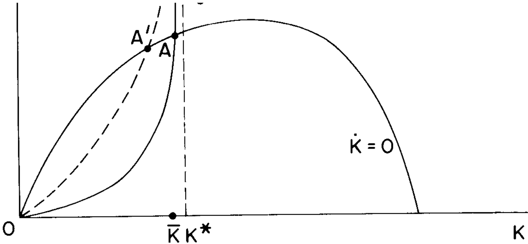
the C ˙ = 0 \dot{C}=0 C ˙ = 0 C ˙ = − d ( d + ϑ ) D \dot{C} = -\pDies(\pDies+\timeRate)D C ˙ = − d ( d + ϑ ) D C C C
C ˙ = 0 \dot{C}=0 C ˙ = 0 C C C C ˙ = 0 \dot{C}=0 C ˙ = 0
locus shifts up (or, equivalently, to the left). Thus, the new
equilibrium will be at a lower value of K K K
rate.
The phase diagram shows that the new equilibrium point A ′ A' A ′
of the original equilibrium. This is because at a given level of the aggregate
capital stock, consumers spend more because W > W \mathcal{W}>W W > W
Ricardian equivalence does not hold in this model, because a tax cut today
financed by a future perpetual tax is a transfer of resources from future
consumers to today’s consumers, and there are no altruistic links that
make current consumers offset this by saving more on behalf of future
generations.
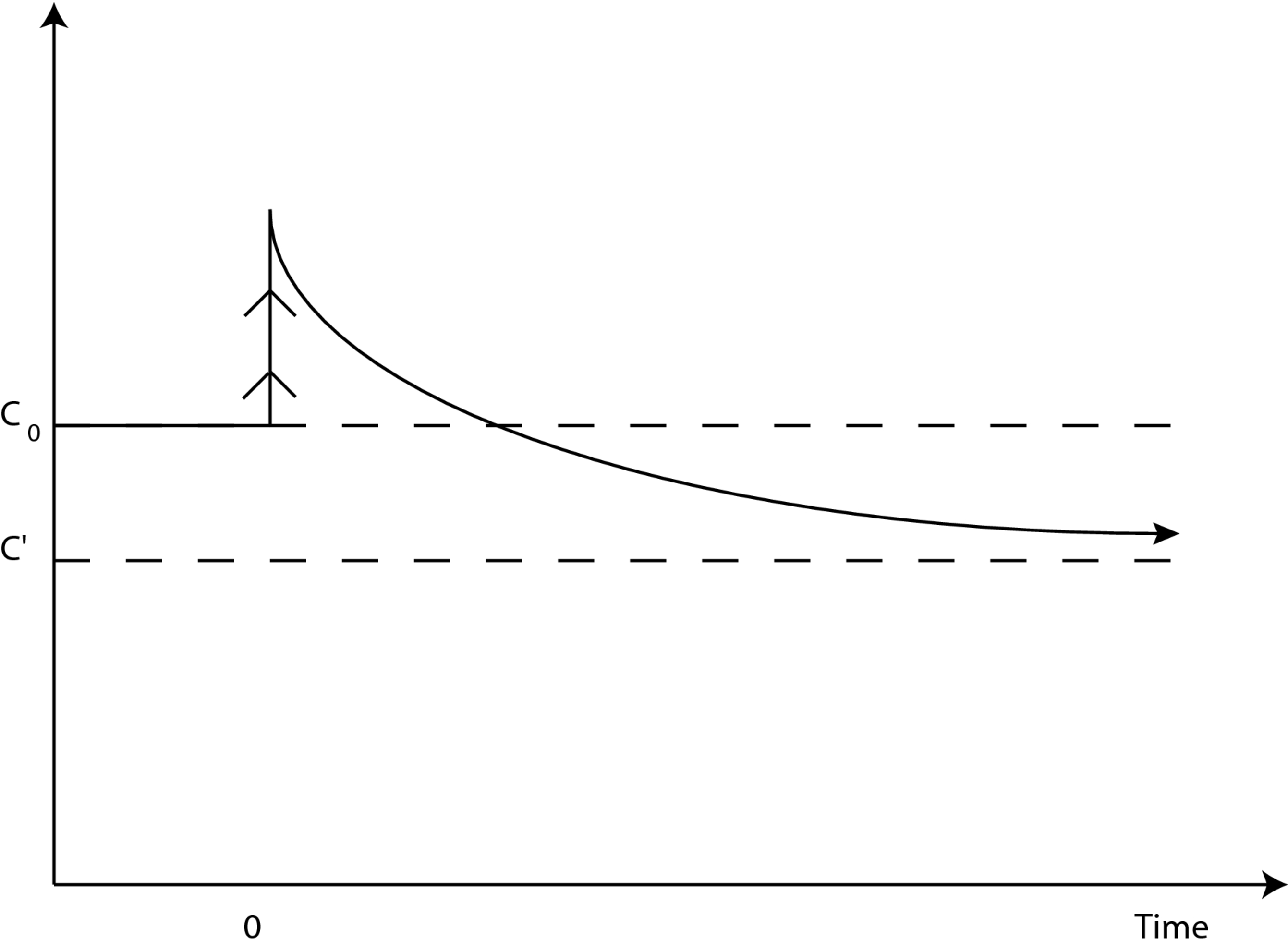
The next figure shows the path of consumption per capita in this
economy. Prior to time 0, the economy was in its steady-state
equilibrium at the level of consumption C 0 C_0 C 0
equilibrium labeled A A A
policy is carried out. The fiscal policy immediately increases
consumption because it amounts to a transfer of resources from future
to current generations. However, the higher level of consumption runs
down the capital stock per capita, and so over time consumption asypmtotically
approaches a new, lower equilibrium level of consumption C ′ C' C ′
Blanchard shows that if the model is changed so that each
consumer’s income declines exponentially at rate γ \gamma γ γ \gamma γ
C ˙ = ( α K α − 1 − δ + γ − ϑ ) C − ( d + γ ) ( d + ϑ ) K K ˙ = K α − δ K − C . \begin{gathered}\begin{aligned}
\dot{C} & = (\alpha K^{\alpha-1}-\delta +\gamma-\timeRate)C-(\pDies+\gamma)(\pDies+\timeRate)K
\\ \dot{K} & = K^{\alpha}-\delta K - C.
\end{aligned}\end{gathered} C ˙ K ˙ = ( α K α − 1 − δ + γ − ϑ ) C − ( d + γ ) ( d + ϑ ) K = K α − δK − C . Note that it is possible to rewrite the C ˙ = 0 \dot{C}=0 C ˙ = 0
( α K α − 1 − δ + γ − ϑ ) C = ( d + γ ) ( d + ϑ ) K \begin{gathered}\begin{aligned}
(\alpha K^{\alpha-1}-\delta +\gamma-\timeRate)C & = (\pDies+\gamma)(\pDies+\timeRate)K
\end{aligned}\end{gathered} ( α K α − 1 − δ + γ − ϑ ) C = ( d + γ ) ( d + ϑ ) K Use this equation to show that as C → ∞ C \rightarrow \infty C → ∞ C ˙ = 0 \dot{C}=0 C ˙ = 0
r = α K α − 1 − δ = ϑ − γ \begin{gathered}\begin{aligned}
\rfree = \alpha K^{\alpha-1} - \delta & = \timeRate - \gamma
\end{aligned}\end{gathered} r = α K α − 1 − δ = ϑ − γ Thus, for a large enough value of γ \gamma γ
Answer:
As C C C (56)
the equation can continue to hold is if
lim C → ∞ ( α K α − 1 − δ + γ − ϑ ) = 0 \begin{gathered}\begin{aligned}
\lim_{C \rightarrow \infty} (\alpha K^{\alpha-1}-\delta +\gamma-\timeRate) & = 0
\end{aligned}\end{gathered} C → ∞ lim ( α K α − 1 − δ + γ − ϑ ) = 0 which implies (57)
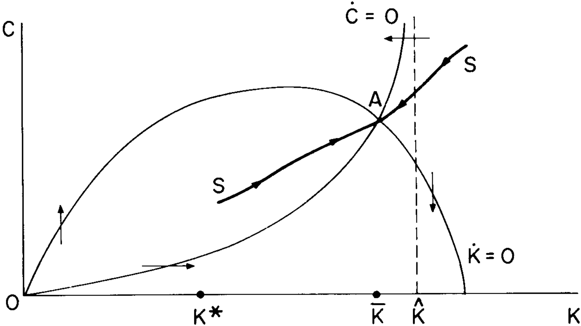
The new phase diagram shows the C ˙ = 0 \dot{C}=0 C ˙ = 0
K ˙ = 0 \dot{K}=0 K ˙ = 0 K ˙ = 0 \dot{K}=0 K ˙ = 0
This is implied by the fact that the net interest rate is negative, which
means that the net interest rate could be increased by reducing
the capital stock.
The reason this is an interesting case is that in this case it is
possible for the economy to be in a condition of dynamic inefficiency,
just as in the 2-period OLG models discussed early in the class. The idea
is to think of declining labor income as a way to generate a ‘life cycle’
saving motive. In such a case the fiscal experiment examined above
is interesting because it could rescue an economy with too much capital
from a state of dynamic inefficiency.
Blanchard, O. J. (1985). Debt, Deficits, and Finite Horizons. Journal of Political Economy , 93 (2), 223–247. 10.1086/261297