Consumption Under Perfect Foresight and CRRA Utility

Two companion notebooks in the Econ-ARK DemARK collection work this model numerically. How Close Is HARK’s Infinite-Horizon Solution? measures how a numerical solution, found by iterating backward from the last period of life, approaches the exact formulas derived here. Perfect Foresight CRRA Model - Saving Rate uses HARK to compute the consumer’s saving rate.

1The Problem¶

This section solves the problem of a perfect foresight consumer with intertemporally separable CRRA utility $\uFunc(\bullet)= \bullet^{1-\CRRA}/(1-\CRRA)$ who discounts future utility geometrically by a factor $\Discount$ per period. The finite horizon solution, whose last period is $\TEnd$, extends to the infinite horizon case if intuitive “impatience” and “finite human wealth” conditions hold.

The consumer’s problem in period $t$ is to

subject to the constraints below, in which we introduce $\bLevBF$ and $\mLevBF$ because it is useful to have a term for the consumer’s non-income resources at the beginning of the period,

where $\pLevBF_{\tNow+1}$ is “permanent labor income,” which always grows by a factor $\WGro$:

2The Solution¶

It will be convenient to think of both market resources $\mLevBF_{\tNow}$ and permanent noncapital (labor) income $\pLevBF_{\tNow}$ as state variables in this problem. Bellman’s equation is^[1]

The first order condition for this maximization is

and the Envelope theorem tells us that

But the right hand sides of (5) and (6) are identical, so

and similar logic tells us that $\vFunc_{\tNow+1}^{\mLevBF}(\mLevBF_{\tNow+1},\pLevBF_{\tNow+1})=\uFunc^{\prime}(\cLevBF_{\tNow+1}),$ which (substituting $\uFunc^{\prime}$ for $\vFunc^{\mLevBF}$ in (6)) gives us the Euler equation for consumption:

Thus, consumption grows in every period by a factor $\Pat \equiv (\Rfree\Discount)^{1/\CRRA}$, where we use the Old English letter $\Pat$ to measure what we will call the “absolute patience” factor. Specifically, if

we will say that the consumer exhibits “absolute impatience” because this is the condition that guarantees that the level of consumption will be falling (and what better definition of absolute impatience could there be than deliberately spending so much that you will have to cut your spending in the future?). If $\Pat > 1$ the consumer exhibits “absolute patience” (the consumer wants to defer resources into the future in order to achieve consumption growth).

The Intertemporal Budget Constraint tells us^[2]

Fact FinSum can be used to show that the PDV of labor income (also called “human wealth” $\hLevBF_{\tNow}$) is

while the PDV of consumption is

We can solve the model by combining (12) and (11) using (10) to obtain:

where $\MPC_{t}$ is the marginal propensity to consume (MPC) out of overall (human plus nonhuman) wealth $\oLev_{t}$.

Human wealth as defined in the PDV of labor income includes the current period’s income: its sum starts at $n=0$. Human wealth from the next period on, called end-of-period human wealth $\hEnd_{t}$ and measured as a ratio to $\pLevBF_{\tNow}$, leaves that income out:

which approaches $({\WGro}/\Rfree)/(1-{\WGro}/\Rfree)$ as $\TEnd \rightarrow \infty$ when the finite human wealth condition below holds.^[3]

In order to apply InfSum to move to the infinite-horizon case ($\TEnd=\infty$), we need to impose the condition

Why? Because if income were expected to grow at a rate greater than the interest rate forever, then the PDV of future income would be infinite; with infinite human wealth, the problem has no well-defined solution. We henceforth call (15) the Finite Human Wealth Condition (FHWC).

Similarly, if consumption starts at a positive level and grows by the factor $\Pat=(\Rfree \Discount)^{1/\CRRA}$, in order for the PDV of consumption to be finite we must impose:

and we will henceforth call $\PatR$ the “return patience factor” whose log is the “return patience rate” $\patr \equiv \log \PatR$ ($\pat$ is the lower-case version of $\Pat$) and what (16) says is that the desired growth rate of consumption must be less than the interest rate in order for the model to have a well-defined solution. This condition therefore imposes a requirement that “impatience” be greater than some minimum amount. (For (much) more on the various definitions of impatience used in this section, their implications, and parallel conditions for models with uncertainty, see Carroll (n.d.)).

If both the RIC and the FHWC hold, then the model has a well-defined infinite horizon solution,^[4] as can be seen by realizing that

Substituting these zeros into (13) yields

where $\oLev_{\tNow}$ is the consumer’s “overall” or “total wealth,” the sum of human and nonhuman wealth, and $\MPC$ is the infinite-horizon marginal propensity to consume.

Now consider the question “What is the level of $\cLevBF_{\tNow}$ that will leave total wealth intact, allowing the same value of consumption in period $t+1$ and forever after (that is, allowing $\cLevBF_{\tNow+n}=\cLevBF_{\tNow}~\forall~n>0$)?”

The intuitive answer is that the wealth-preserving level of spending is exactly equal to the (properly conceived) interest earnings on one’s total wealth. We call this the “sustainable” level of consumption. The literature of the 1970s and 80s interpreted that quantity as “permanent income,” but we reserve that term here for $\pLevBF$ itself. Wealth in this framework behaves exactly like an asset that yields a dividend $\pLevBF$.

Because human wealth is exactly like any other kind of wealth in this perfect foresight framework, it is possible to work directly with the level of total wealth $\oLev$ to find the sustainable level of spending. Suppose we assume the consumer will spend fraction $\PIHMPC$ of total wealth in each period; the $\PIHMPC$ that leaves wealth intact will be given by $\PIHMPC$ in

Thus, the consumer can spend only the interest earnings $\rfree$ on wealth, divided by the return factor $\Rfree$. (The division occurs because the requirement is to be able to spend the same amount next period, so you need to account for the time cost of today’s spending by dividing by $\Rfree$ which connects today’s spending to tomorrow’s wealth.)

Note that the coefficient multiplying total wealth in (18) is also divided by $\Rfree$. Thus, whether the consumer is spending more than the sustainable amount, exactly the sustainable amount, or less than the sustainable amount depends upon whether the numerator in (18) is greater than, equal to, or less than $\rfree$. As noted before, the consumer will be “absolutely impatient” if

Finally, if $\Rfree\Discount=1$ (which is to say, the interest rate exactly offsets the time preference rate), then $(\Rfree\Discount)^{1/\CRRA}=1$ regardless of the value of $\CRRA$ so that the consumer is “poised” on the knife-edge between patience and impatience. We refer to such a consumer as “absolutely poised.” Similarly, we say that a consumer for whom $\PatR=1$ is “return poised.”

The two conditions do different work. Return impatience guarantees a positive marginal propensity to consume, while absolute impatience guarantees a falling level of consumption. Whenever $\rfree > 0$, return impatience holds even for a consumer who is poised with respect to absolute patience.

(The consumer will be impatient, spending more than his income, if $\Rfree\Discount<1$, and patient, spending less than his income, if $\Rfree\Discount>1$. Income here means income inclusive of the interest earnings on total wealth.)

Equation (18) can be simplified into something a bit easier to handle by making some approximations. If $\Discount = 1/(1+\timeRate)$, then we can use facts from the MathFacts section to discover that

Substituting this into (18) gives

The consumption function (18) is exact; (22) treats $\rfree$, $\timeRate$ and the return patience rate $\patr$ as small. Its error is a different thing from the error of a numerical solution, which approaches the exact formula, not the approximation.

From this we can see again that whether the consumer is return patient, return poised, or return impatient depends on the relationship between $\rfree$ and $\timeRate$. Note also that if $\CRRA = \infty$ then the consumer is infinitely averse to changing the level of consumption, and so once again the consumer spends exactly the sustainable amount. (This consumer is “absolutely poised” but “return impatient”).

Now a brief digression on what “income” means in this model. Suppose for simplicity that the consumer had no capital assets (“bank balances” $\bLevBF_{\tNow}=0$), and suppose that income was expected to stay constant at level $\pLevBF_{\tNow+n}=\pLevBF~\forall~n>0$ forever. In this case human wealth would be:

We found in equation (19) that the level of consumption that leaves “wealth” $\oLev_{\tNow}$ intact was

So in this case, spending the “interest income on human wealth” corresponds to spending exactly your labor income. This seems less mysterious if you think of income $\pLevBF_{\tNow}$ as the “return” on your human capital, which is an asset whose value is $\hLevBF_{\tNow}$. If you “capitalize” your stream of income using the interest factor $\Rfree$ and then spend the interest income on the capitalized stream, it stands to reason that you are spending the flow of income from that source.

With constant $\pLevBF$ we can rewrite (22) as

$\rfree$ appears three times in this equation. In order, the three appearances are the income effect, the substitution effect and the human wealth effect, as the two-period model defines them. The first two are inside the marginal propensity to consume out of total wealth, so they are the effects of $\rfree$ on consumption for a given total wealth $\bLevBF_{\tNow}+\hLevBF_{\tNow}$. An increase in the first $\rfree$ raises the payout rate on total wealth (set $\pLevBF = 0$ and use (19) for $\PIHMPC$, with $\rfree/\Rfree \approx \rfree$ for small $\rfree$): this is the income effect. The second is the substitution effect, as its dependence on the intertemporal elasticity of substitution $\CRRA^{-1}$ shows. The third, in $\pLevBF(\Rfree/\rfree)$, is the human wealth effect: the effect of $\rfree$ on human wealth itself, which comes from the budget constraint and involves no preference parameter. Bank balances $\bLevBF_{\tNow}$ are in none of the three; they are part of the total wealth that the marginal propensity to consume applies to. Because consumption depends on $\bLevBF_{\tNow}$ and $\hLevBF_{\tNow}$ only through their sum, this formula, like the two-period model, assumes that the consumer can borrow against future income at no penalty. How Large is the Human Wealth Effect? measures what the human wealth effect does to consumption under that assumption.

3Normalizing By $\pLevBF$¶

The whole problem can be restated more simply by “dividing through” by the level of permanent income before solving. Hereafter, nonbold variables will be the normalized bold-letter equivalent, e.g. $\cRat_{\tNow}=\cLevBF_{\tNow}/\pLevBF_{\tNow}$, and note that if $\pLevBF_{\tNow+1}={\WGro} \pLevBF_{\tNow}~\forall~t$ then from the standpoint of date $t$,

which means that

Furthermore, the accumulation equations can be rewritten by dividing both sides by $\pLevBF_{\tNow+1}$:

Now if we define $\DiscAlt \equiv {\WGro}^{1-\CRRA}\Discount$ and $\RnormWGro \equiv \Rfree/{\WGro}$, the original problem can be rewritten as:

subject to the constraints

and we can go through the same steps as above to find that the solution is

subject to the “finite human wealth” condition

which is the same condition (15) as above, and also subject to the “return impatience condition”

which is also the same as above in (16).

Now note that (32) can be rewritten

where $\oRat_{\tNow}$ is the consumer’s total wealth-to-permanent-labor-income ratio, and $\MPC$ is the “marginal propensity to consume” out of wealth.

As before, whether $\oRat$ is rising or falling depends upon the relationship between $\RnormWGro-1$ and $\RnormWGro-(\RnormWGro\DiscAlt)^{1/\CRRA}$. A consumer will be drawing down his wealth-to-income ratio if

Now substituting the definitions of $\RnormWGro$ and $\DiscAlt$ we see that whether $\oRat$ is rising or falling depends on whether

where $\PatWGro$ is the “growth patience factor.” We call (37) the “growth impatience condition” (GIC),^[5] and we say that the consumer is “growth impatient” if (37) holds.

Thus, whether the consumer is patient or impatient in the sense of building up or drawing down a wealth-to-income ratio depends on whether the growth rate of labor income is less than, equal to, or greater than the growth rate of consumption. Analogously to our earlier usages, a consumer for whom $\PatWGro=1$ (equivalently, $\patwGro= 0$) would be “growth poised.”

To get the intuition for this, consider the case of a consumer with no nonhuman wealth, $\bRat_{\tNow}=0$. This consumer’s absolute level of consumption will grow at $(\Rfree\Discount)^{1/\CRRA}$ and absolute level of income grows at ${\WGro}$, but the PDV of future consumption and future income must be equal. If income is growing faster than consumption but has the same PDV, consumption must be starting out at a level higher than income, which is the sense in which this consumer is impatient (spending more than his income). “Growth impatience” is therefore the condition that causes consumers with no assets to want to borrow.

4Applications¶

4.1How Large is the Human Wealth Effect?¶

We can now apply the model to answer our first useful question: How large does the model imply the “human wealth effect” is?

For simplicity, assume that $\bRat_{\tNow} = 0$. Then the original version of the approximate formula (22) tells us that the level of consumption will be given by:

We are interested only in calibrations of the model in which the consumer is “growth impatient” so that $\wGro > \CRRA^{-1}(\rfree-\DiscRate)$ so if we define the growth patience rate as

we can write this as

Remembering that imposition of the growth impatience condition is equivalent to assuming $\patwGro < 0$, while the FHWC requires $\rfree > \wGro$, it is clear that the expression $-\patwGro/(\rfree-\wGro)$ will be positive: The consumer will spend more than his permanent labor income.

Now suppose we choose plausible values for $(\rfree, \timeRate, \wGro, \CRRA) = (0.04,0.04,0.02,2)$. Then (38) becomes:

Now suppose the interest rate changes to $\rfree=0.03$, while all other parameters remain the same. Then (38) becomes:

The point of this example is that for plausible parameter values, the human wealth effect is enormously stronger than the income and substitution effects, so that we should see large drops in consumption when interest rates rise and conversely strong gains when interest rates fall. This is a summary of the main point of the famous paper by Summers (1981); Summers derives formulas for an economy with overlapping generations of finite-lifetime consumers, but those complications do not change the basic message.

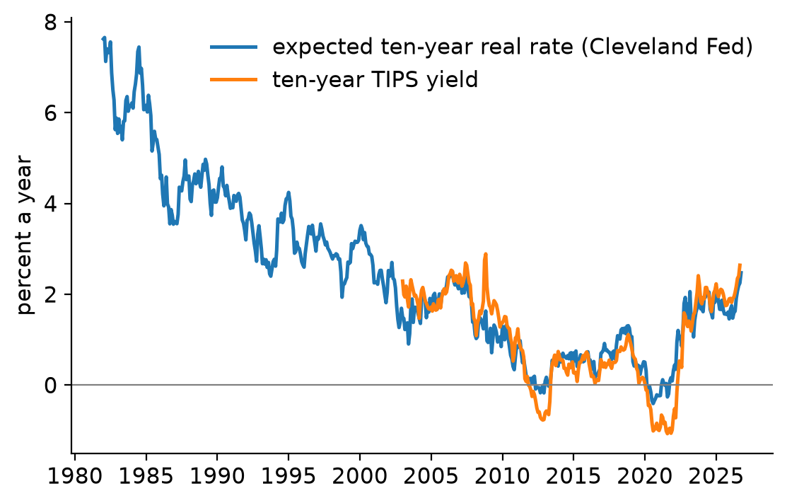
Nor is a change of a percentage point in the long-term real interest rate unusual. The long-term real interest rate figure shows two measures of it. One is the Federal Reserve Bank of Cleveland’s estimate of the real rate expected over the next ten years, from a model fitted to Treasury yields, inflation, inflation swaps and surveys of expected inflation Haubrich et al., 2012. The other is the yield on ten-year inflation-indexed Treasury bonds (TIPS). The expected rate averaged 5.3 percent a year in the 1980s and 0.6 percent in the 2010s, and reached a low of −0.4 percent in August 2020. The TIPS yield rose by 3.5 percentage points in two years, from −1.07 percent in August 2021 to 2.41 percent in October 2023. Since 1982 the expected rate has moved by a percentage point or more within a year in 13 percent of months, and within two years in 24 percent. The notebook computes these numbers from FRED’s data; open it in Colab or Binder to run it without installing anything.

4.2How Does the Saving Rate Respond to Interest Rates?¶

The level of saving can be defined as total income minus total consumption:

but substituting from (40) and (22),

this can be rewritten as

(where the last approximations come from the assumptions that $1/G \approx 1$) and that $\rfree \times (\rfree-\CRRA^{-1}(\rfree-\DiscRate))$ is “small.” The saving rate (for which we use the letter $\srate$ to distinguish it from $\sRat$ above) is the ratio of saving to total income (not just labor income):

The first thing to notice about this expression is that as $\aRat_{\tNow-1}$ approaches infinity, the saving rate asymptotes to

and whether the saving rate is positive or negative depends on whether the consumer is absolutely impatient, absolutely poised, or absolutely patient.^[6]

Finally, if we rewrite this as

then it is apparent that the response of the saving rate to the interest rate is

If we consider almost any plausible configuration of parameter values, say $\rfree = \timeRate=0.05$ and $\CRRA = 2$, this translates to a very large response of the saving rate with respect to $\rfree$ (in the case of the parameter values mentioned above, $(1/2)(20)=10$).

5Appendix¶

5.1The Limiting Solution to the Perfect Foresight Model if the FHWC Fails¶

5.1.1When the RIC Holds¶

Consider first a circumstance in which the RIC holds ($\PatR<1$). In this case, the perfect foresight unconstrained model does not have a sensible solution because human wealth is infinite while the model implies that the optimal policy is to consume a positive proportion of human wealth. $\cFunc(\mRat)=\infty~\forall~\mRat$ is not a useful (or plausible!) solution.

5.1.2When the RIC Fails¶

The alternative case is when the RIC fails ($\PatR>1$). Here, the only way to make sense of the model is to think about the limit of the finite horizon model as the horizon extends to infinity. This is because behavior reflects a competition between two pathologies that characterize the infinite horizon solution: It exhibits a limiting MPC of zero out of total wealth, which includes human wealth, which approaches infinity. A limiting solution of $\cFunc(\mRat) = 0 \times \infty$ is even less useful than $\cFunc(\mRat) = \infty$!

It turns out that the limiting solution is not ambiguous, however. The finite horizon solution implies that consumption out of human wealth when the end of life is $n$ periods in the future is

whose limit is given by

since when the RIC fails and the FHWC also fails ($\WGro > \Rfree$), both the numerator and the denominator diverge, so the limit is governed by the ratio of the dominant terms. That ratio is infinite as long as the growth patience factor satisfies $\PatWGro < 1$, in which case $\PatWGro^{n+1}$ approaches zero as $n \uparrow \infty$. (In the case treated above, where the RIC holds rather than fails, $\PatWGro<1$ follows automatically, because $\Pat < \Rfree$ and $\Rfree < \WGro$ together imply the GIC $\Pat < \WGro$.)

5.2Useful Analytical Results¶

Given the result from (8) that

we can rewrite the value function as

but since $\DiscFac \Pat^{1-\CRRA} = \PatR$,^[7] this reduces to

where $\cPDVFunc_{t}$ is the discounted value of future consumption growth (that is, the discounted value of the ratio of future consumption to today’s consumption).

Carroll (n.d.) shows (in an appendix) that $\cPDVFunc_{t} = \MPC_{t}^{-1}$, which means that we can write value as

5.3Additional Derivations¶

If consumption is simply a function of overall wealth bank balances $\oRat_{t}$, we can derive a convenient recursive formula for the inverse of the MPC:

which implies that if the MPC in the last period $T$ is $\MPC_{T}=1$ then from any date $t \leq T$ we can write

But the series on the RHS in (54) and (57) are identical! So $\MPC^{-1}_{t} = \cPDVFunc_{t}$, and we can equivalently write

Now note that if we define a utility-inverse of the value function as $\vInv \equiv \left((1-\CRRA) \vFunc\right)^{1/(1-\CRRA)}$, then consumption exceeds its minimum possible value at $\underline{\mRat}$ (where consumption exceeds $\cFunc(\underline{\mRat})=0$) by $c_{t}=\MPC_{t}(\mRat-\underline{m})$:

which is linear, and makes it very easy to compute

References

1. Carroll, C. D. (Forthcoming). Theoretical Foundations of Buffer Stock Saving. Quantitative Economics. 10.5281/zenodo.4088917
2. Summers, L. H. (1981). Capital Taxation and Accumulation in a Life Cycle Growth Model. American Economic Review, 71(4), 533–544.
3. Haubrich, J., Pennacchi, G., & Ritchken, P. (2012). Inflation Expectations, Real Rates, and Risk Premia: Evidence from Inflation Swaps. Review of Financial Studies, 25(5), 1588–1629. 10.1093/rfs/hhs003