The decentralization of the Ramsey/Cass-Koopmans model showed that an economy of many households behaves exactly like a single representative household, provided every household is identical and can insure any risk at an actuarially fair rate. Real households face large uninsurable risks to their own incomes, that are mostly unrelated to what happens to everyone else in the economy.[1] A prudent household facing such risk saves for precautionary reasons, and buffer stock models show how much. This chapter asks what happens when a whole economy consists of such households, and their saving sets the interest rate and the wage.
Aiyagari (1994) asked by how much uninsurable idiosyncratic risk raises the capital stock and the saving rate. For his parameter values, the answer was “not by much.” The interest of the model lies in why.
1From Friedman to Bewley to Aiyagari
Friedman (1957) argued that consumption depends on permanent income, and that measured income is permanent income plus a transitory component that consumers largely save or dissave. The argument was in words, not in math. Muth (1960) mathematized it: when income is a random walk plus serially uncorrelated noise, the best forecast of future income is an exponentially weighted average of past income, which is actually exactly how Friedman had proposed to measure permanent income. Hall (1978) later showed that, under certainty equivalence, consumption follows a random walk (see random walk and consumption function).
Certainty equivalence rules out precautionary saving. Dropping it, when utility is not quadratic, leaves a problem with no closed-form solution. Bewley (1977) formulated the permanent income hypothesis for a single infinitely lived consumer who cannot borrow against random income, and Bewley (1986) placed a continuum of such consumers, with independent shocks, in a general-equilibrium exchange economy. Zeldes (1989) and Deaton (1991) solved such problems numerically, and Carroll (1992) calibrated one to household income in the Panel Study of Income Dynamics (PSID) and argued that precautionary motives quantitatively explain the behavior of aggregate consumption over the business cycle. Following Deaton, Carroll termed such behavior buffer stock saving.
Huggett (1993) used such households to determine the interest rate on a bond in zero net supply. Aiyagari (1994) put them into the neoclassical growth model, so that their saving becomes the capital stock. Models of this kind are now called “Aiyagari models,” and his paper is the reference point for whether idiosyncratic risk matters for aggregates.
2The Household’s Problem
Each of a continuum of households, of total mass one, maximizes
with . It supplies an exogenous, random endowment of labor at the wage and holds assets earning the interest rate , so its market resources evolve as
where is end-of-period assets and is the borrowing limit.
The idiosyncratic labor productivity component is the only source of risk. Its logarithm follows a first-order autoregression with persistence ,
so is the unconditional standard deviation of . For computation the process becomes a finite Markov chain (Tauchen (1986)). With a continuum of households, the cross-section distribution of endowments is always the chain’s stationary distribution, though each household’s endowment keeps moving.
The Euler equation now holds with equality only when the household is not at its borrowing limit:
The solution is a consumption function for each level of the endowment, . In the consumption functions figure, each follows the 45-degree line until the household prefers to save, and is concave beyond. A household with a low endowment spends less at a given , because a low wage today forecasts low wages to come.
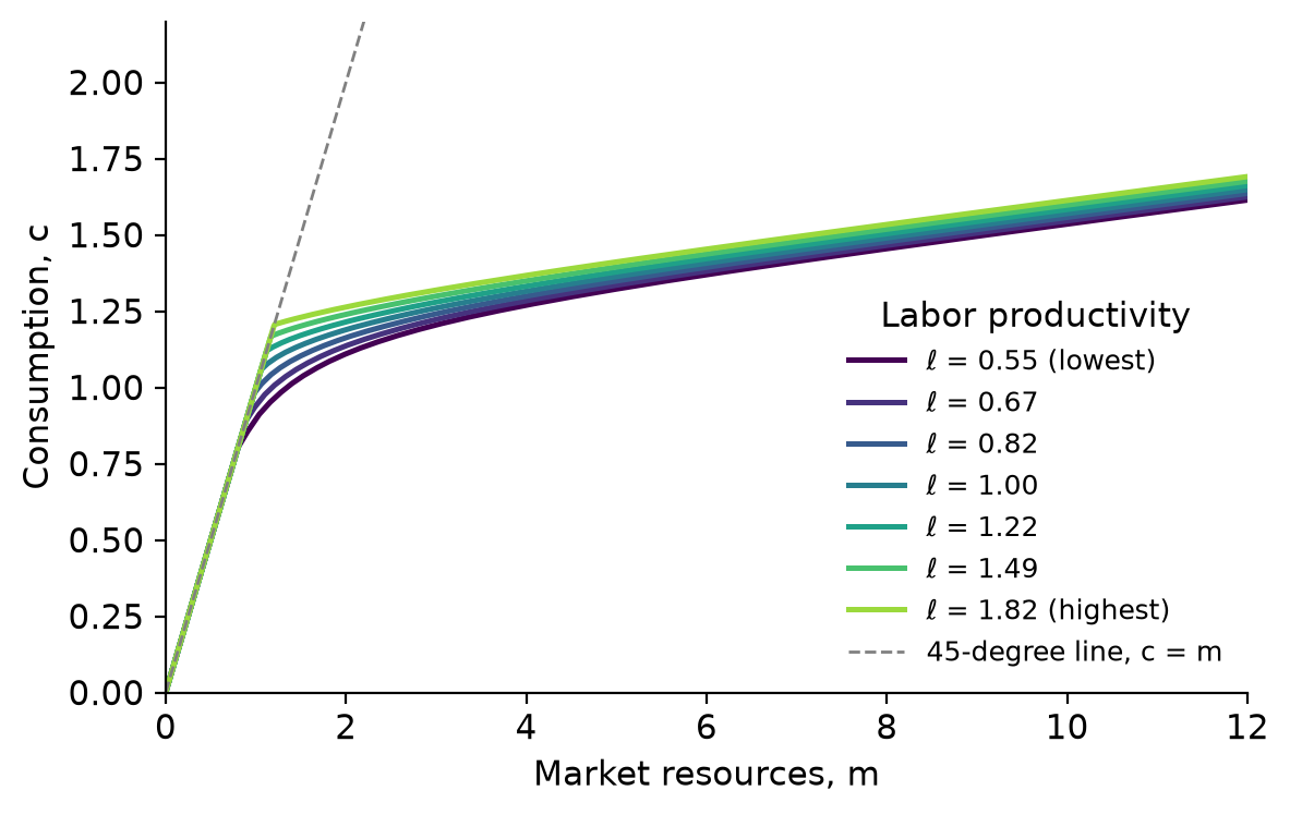
Figure 1:The consumption function for each of the seven levels of the idiosyncratic labor productivity component, from lowest (dark) to highest (light), at the equilibrium interest rate for Aiyagari’s baseline: , , , , and no borrowing.
2.1How Much May a Household Borrow?
If the endowment never falls below some and , the most a household can repay for certain is the present discounted value of the worst possible stream of wages.
A household never borrows all the way to this limit: a run of the worst endowment would leave it nothing to consume, which CRRA utility makes infinitely costly. Aiyagari’s baseline of no borrowing, , is tighter.
2.2Why Wealth Stays Bounded
The perfect foresight conditions carry over. Return impatience makes the household’s problem well defined, and growth impatience keeps wealth bounded relative to income. Income does not grow here, so growth impatience is , or ; it coincides with absolute impatience only for that reason. With , as in Aiyagari’s most extreme calibration, human wealth is infinite and only the borrowing limit keeps the problem well defined. If , consumption and assets grow without bound for almost every household (Chamberlain & Wilson (2000)).
3Firms and Factor Prices
Competitive firms produce with , and capital depreciates at rate . As in the decentralized Ramsey model, the interest rate households earn is the marginal product of capital net of depreciation, and the wage is the marginal product of labor; with aggregate labor ,
Inverting the first gives the capital firms want at each interest rate,
a downward-sloping demand curve. The wage moves with the interest rate, so the interest rate affects saving both directly and through the wage.
4Stationary Equilibrium
Each household’s circumstances keep changing; only the distribution is constant. Write for mean assets in the stationary distribution at the interest rate and the wage it implies.
With complete markets, the economy would have the Ramsey/Cass-Koopmans steady state: , a horizontal supply of capital at that rate, and an indeterminate distribution of wealth across households. With uninsurable risk, households would accumulate without limit at , so the interest rate must be lower. Averaging the Euler equations shows this directly.
Here is the slack in the Euler equation, positive only at the limit, and in a stationary distribution the average of equals that of .
In the capital supply and demand figure, supply rises without bound as approaches , and crosses demand at a lower interest rate and a higher capital stock than complete markets give. General equilibrium limits the effect: the extra capital drives the interest rate down, which makes saving less attractive.
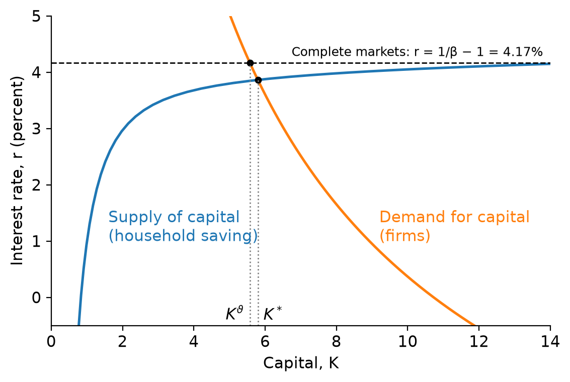
Figure 2:Steady-state supply and demand for capital, with the wage moving with the interest rate. With complete markets the supply of capital is horizontal at the time preference rate , and the capital stock is ; with uninsured idiosyncratic risk it is . Baseline parameters as in the consumption functions figure.
Nothing guarantees that supply slopes up everywhere, so the equilibrium need not be unique (Açıkgöz (2018)); Light (2020) and Achdou et al. (2022) prove uniqueness only under conditions that include relative risk aversion no greater than one.
5Gross Saving and Net Saving
Aiyagari measured saving gross. Investment, including the replacement of worn-out capital, is divided by output measured before depreciation, so capital’s income in the denominator is . In a steady state without growth, investment just replaces depreciation:
This is the gross saving rate of the growth model. The consumption chapters of this book instead study net saving: the household’s income includes interest at , already net of depreciation (), and saving is that income minus consumption. In Aiyagari’s steady state net saving is zero, in the aggregate and for the average household: the saving of households building their buffers is matched by the dissaving of households drawing them down. Precautionary motives raise the capital stock, and a larger capital stock needs more replacement investment, which is why they raise the gross saving rate.
6Computing the Equilibrium
Aiyagari’s algorithm repeats three steps until the interest rate settles down:
Guess an interest rate , and compute the wage from the firms’ first-order conditions.
Solve the household’s problem at those prices, and simulate one household for many periods (Aiyagari used 10,000) to find mean assets .
If exceeds , lower the guess; if it falls short, raise it.
The notebook carries out these steps with the code of the Aiyagari1994QJE REMARK, which builds the households with HARK and, like Aiyagari, simulates them; open it in Colab or Binder to run it without installing anything.
7Results
A period is a year; Aiyagari set , and (Prescott (1986)), so that with complete markets percent and the saving rate is 23.67 percent. He varied (0.2, 0.4), (0 to 0.9) and (1, 3, 5), with no borrowing. In the baseline (, , ), uninsured risk lowers the interest rate to 3.86 percent (Aiyagari found 3.88), raises capital by 4.0 percent and the saving rate to 24.28 percent. Aiyagari concluded that for moderate risk aversion, variability and persistence the saving rate rises by at most about three percentage points; only when income is both volatile and persistent is the effect large (, , : a negative interest rate and a saving rate of 37.6 percent).
8What the Calibration Leaves Out
8.1The Income Process
Aiyagari’s values of came from first-order autoregressions for individual earnings, such as a working-paper version of Heaton & Lucas (1996), which put it at about 0.2 to 0.5. Panel studies of earnings found a different structure: Abowd & Card (1989) showed that year-to-year changes in log earnings follow a low-order moving average, as Muth’s random walk plus transitory noise implies, and using total family income Carroll (1992) estimated standard deviations of about 0.16 for the annual transitory shock and 0.13 for the permanent one, with a probability of about half a percent a year that family income falls nearly to zero. An autoregression fitted to income of that kind misreads it: the transitory shock acts as measurement error and biases the estimated persistence toward zero. Allowing for it, with an autoregression plus a first-order moving-average error, gives persistence near one: Storesletten et al. (2004) estimate 0.98 to one, and Heathcote et al. (2009) attribute the low estimates of some early studies to the omitted transitory shock.
This matters because the effect of risk on saving rises steeply with persistence; Aiyagari noted that a unit root would lower the interest rate and raise saving enormously. He kept the endowment stationary because, with infinitely lived households and permanent shocks, the cross-section distribution of income would spread out without limit. A constant probability of death, as in Blanchard’s model, keeps it stationary; Carroll et al. (2017) use it to give households permanent and transitory shocks of the sizes the evidence suggests.
8.2The Lowest Income Level
With an endowment bounded away from zero, the natural borrowing limit depends on , a by-product of the discretization rather than an estimate; Aiyagari showed that permitting more borrowing lowers the capital stock. If income can fall to zero with a small probability, as in the PSID, the natural limit is zero: no household borrows if it might have to repay out of nothing, so no borrowing follows from preferences rather than from an arbitrary restriction.
8.3The Distribution of Wealth
The model’s wealth distribution is far more equal than the data’s, across the whole range of the Lorenz curve figure. In the 2004 Survey of Consumer Finances the poorest 40 percent of households hold about 1 percent of net worth, and the poorest fifth slightly less than nothing; in the model the poorest 40 percent hold 15 percent. At the top, the richest 1 percent hold about 32 percent of U.S. net worth but 4 percent in the model, and the Gini coefficients are 0.80 and 0.38. Stachurski & Toda (2019) show that this is no accident of calibration: when infinitely lived households save only in a risk-free asset and share a discount factor, the upper tail of wealth can be no thicker than that of income.
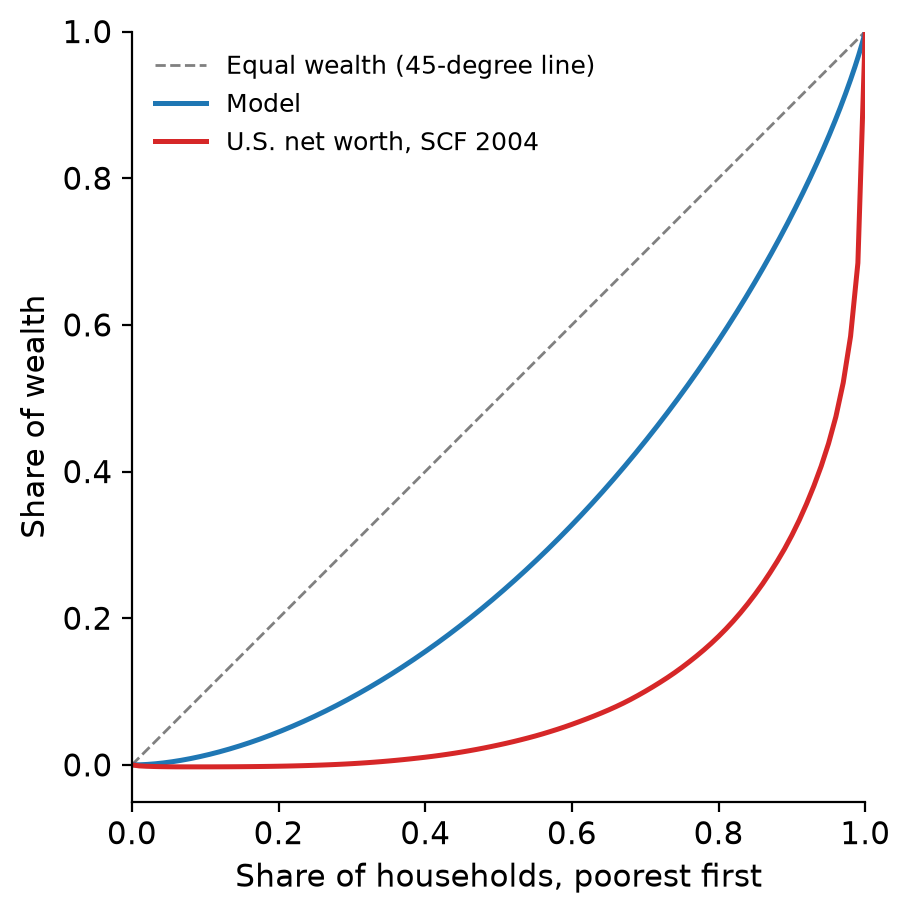
Figure 3:Lorenz curves for wealth: in the baseline Aiyagari economy, and for U.S. net worth in the 2004 Survey of Consumer Finances, the data used by Carroll et al. (2017).
Identical, infinitely lived households all have time to accumulate a large buffer, and that matters for spending. Only about a quarter of one percent of households are at the borrowing limit, and the average annual marginal propensity to consume is 0.054, not far above the perfect foresight value of 0.038 at the same interest rate. Empirical estimates are several times larger; Carroll et al. (2017) show that matching the observed wealth distribution, with its many households holding little, brings the model close to them.
9Why the Answer Came Out as It Did
Aiyagari’s conclusion was widely read as evidence that heterogeneity can be set aside for questions about aggregates. But it follows from his assumptions: households with stationary, moderately persistent income and infinite horizons all hold several years’ income in wealth, a buffer large enough that a bad year barely moves their spending, so they behave much like a representative household. Models that match the evidence on income dynamics and wealth (Carroll et al. (2017); Kaplan et al. (2018)) find that the distribution of wealth matters a great deal for aggregate spending.
10Beyond the Steady State
The model has no aggregate shocks. Krusell & Smith (1998) added them, and found that households forecasting aggregate capital from its mean alone were almost exactly right (“approximate aggregation”), for the same reason as Aiyagari’s result. More recent methods linearize the economy’s response to aggregate shocks around its steady state (Auclert et al. (2021)), making realistic heterogeneity practical in heterogeneous-agent New Keynesian models (Kaplan et al. (2018)).
11Replication
Econ-ARK’s replication of Aiyagari (1994) is the Aiyagari1994QJE REMARK; its econ-ark.org page launches its notebooks in the browser.
Graduate students might consider whether anyone has offered them an insurance contract offering them a guarantee that they will receive the mean average income of the members of their cohort of economics PhD students.
- Aiyagari, S. R. (1994). Uninsured Idiosyncratic Risk and Aggregate Saving. Quarterly Journal of Economics, 109, 659–684. 10.2307/2118417
- Friedman, M. A. (1957). A Theory of the Consumption Function. Princeton University Press.
- Muth, J. F. (1960). Optimal Properties of Exponentially Weighted Forecasts. Journal of the American Statistical Association, 55(290), 299–306. 10.1080/01621459.1960.10482064
- Hall, R. E. (1978). Stochastic Implications of the Life-Cycle/Permanent Income Hypothesis: Theory and Evidence. Journal of Political Economy, 86(6), 971–987. 10.1086/260724
- Bewley, T. (1977). The Permanent Income Hypothesis: A Theoretical Formulation. Journal of Economic Theory, 16(2), 252–292. 10.1016/0022-0531(77)90009-6
- Bewley, T. F. (1986). Stationary Monetary Equilibrium with a Continuum of Independently Fluctuating Consumers. In W. Hildenbrand & A. Mas-Colell (Eds.), Contributions to Mathematical Economics in Honor of Gérard Debreu (pp. 79–102). North-Holland.
- Zeldes, S. P. (1989). Optimal Consumption with Stochastic Income: Deviations from Certainty Equivalence. Quarterly Journal of Economics, 104(2), 275–298. 10.2307/2937848
- Deaton, A. (1991). Saving and Liquidity Constraints. Econometrica, 59(5), 1221–1248. 10.2307/2938366
- Carroll, C. D. (1992). The Buffer-Stock Theory of Saving: Some Macroeconomic Evidence. Brookings Papers on Economic Activity, 1992(2), 61–156. 10.2307/2534582
- Huggett, M. (1993). The Risk-Free Rate in Heterogeneous-Agent Incomplete-Insurance Economies. Journal of Economic Dynamics and Control, 17(5–6), 953–969. 10.1016/0165-1889(93)90024-M
- Tauchen, G. (1986). Finite State Markov-Chain Approximations to Univariate and Vector Autoregressions. Economics Letters, 20(2), 177–181. 10.1016/0165-1765(86)90168-0
- Chamberlain, G., & Wilson, C. A. (2000). Optimal Intertemporal Consumption under Uncertainty. Review of Economic Dynamics, 3(3), 365–395. 10.1006/redy.2000.0098
- Açıkgöz, Ö. T. (2018). On the Existence and Uniqueness of Stationary Equilibrium in Bewley Economies with Production. Journal of Economic Theory, 173, 18–55. 10.1016/j.jet.2017.10.006
- Light, B. (2020). Uniqueness of Equilibrium in a Bewley–Aiyagari Model. Economic Theory, 69(2), 435–450. 10.1007/s00199-018-1167-z
- Achdou, Y., Han, J., Lasry, J.-M., Lions, P.-L., & Moll, B. (2022). Income and Wealth Distribution in Macroeconomics: A Continuous-Time Approach. Review of Economic Studies, 89(1), 45–86. 10.1093/restud/rdab002